CS-466/566: Math for AI

Module 02: Computational Linear Algebra-1

Dr. Mahmoud Mahmoud

The University of Alabama

2026-03-23

TABLE OF CONTENTS

1. Introduction●

2. Tool 1: Norms and Distance○

3. Tools 2: Inner Products○

4. Tools 3: Orthogonality and Projections○

5. Orthonormal Bases○

6. Matrix Properties○

• What is the Determinant?

• What is a Matrix Inverse?

• Change of Basis

10. Gram–Schmidt Algorithm○

Motivation: Why Geometry Matters in ML

Data lives in vector spaces. Learning depends on distance, similarity, and direction.

Geometry explains:

• Clustering
• Cosine similarity
• PCA / projections

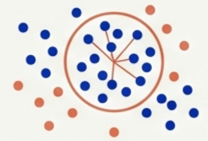
Geometry gives meaning to the data.

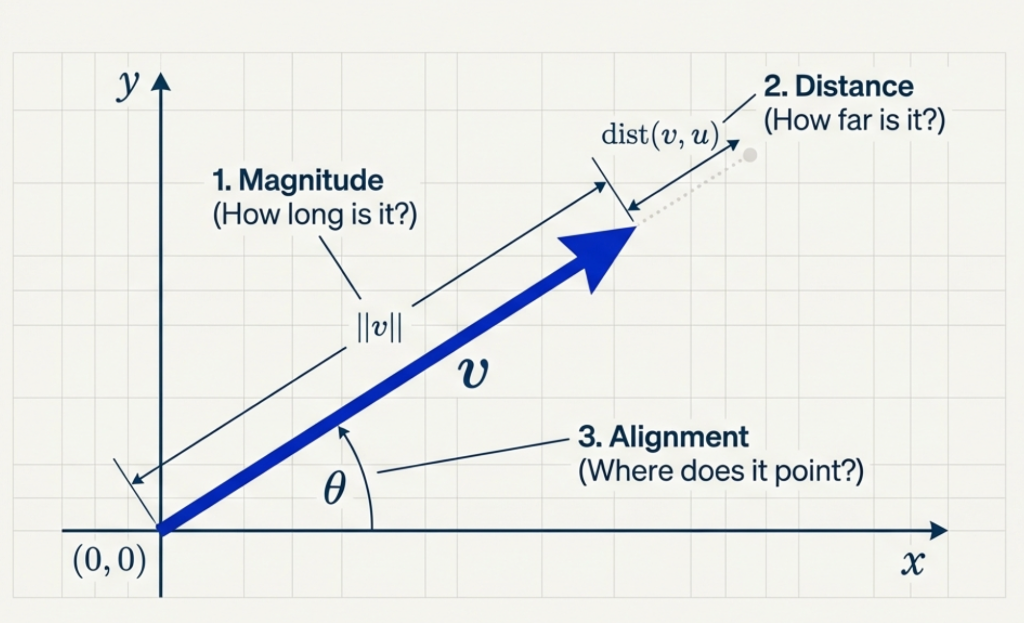
Vectors as Geometry

• A vector is an arrow from the origin
• Geometry asks:
  • How long is it?
  • How far apart are two vectors?
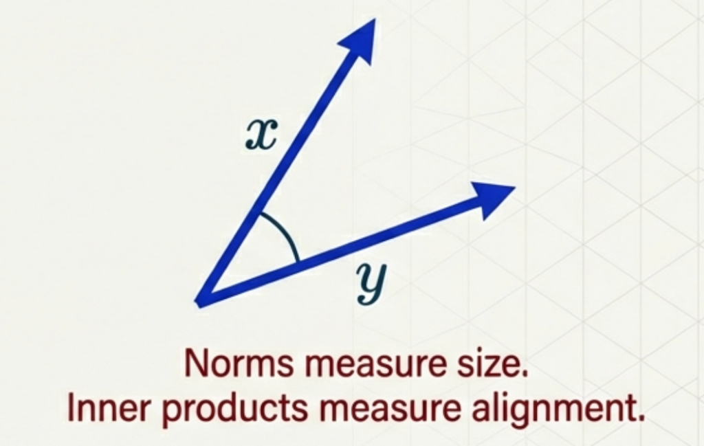
  • How aligned are they?

These questions lead to norms and inner products.

TABLE OF CONTENTS

1. Introduction✓

2. Tool 1: Norms and Distance●

3. Tools 2: Inner Products○

4. Tools 3: Orthogonality and Projections○

5. Orthonormal Bases○

6. Matrix Properties○

• What is the Determinant?

• What is a Matrix Inverse?

• Change of Basis

10. Gram–Schmidt Algorithm○

Norms: Measuring Size

A norm is a function that takes a vector and returns a non-negative number: \(V \to [0,\infty)\)

\[\|x\| \]

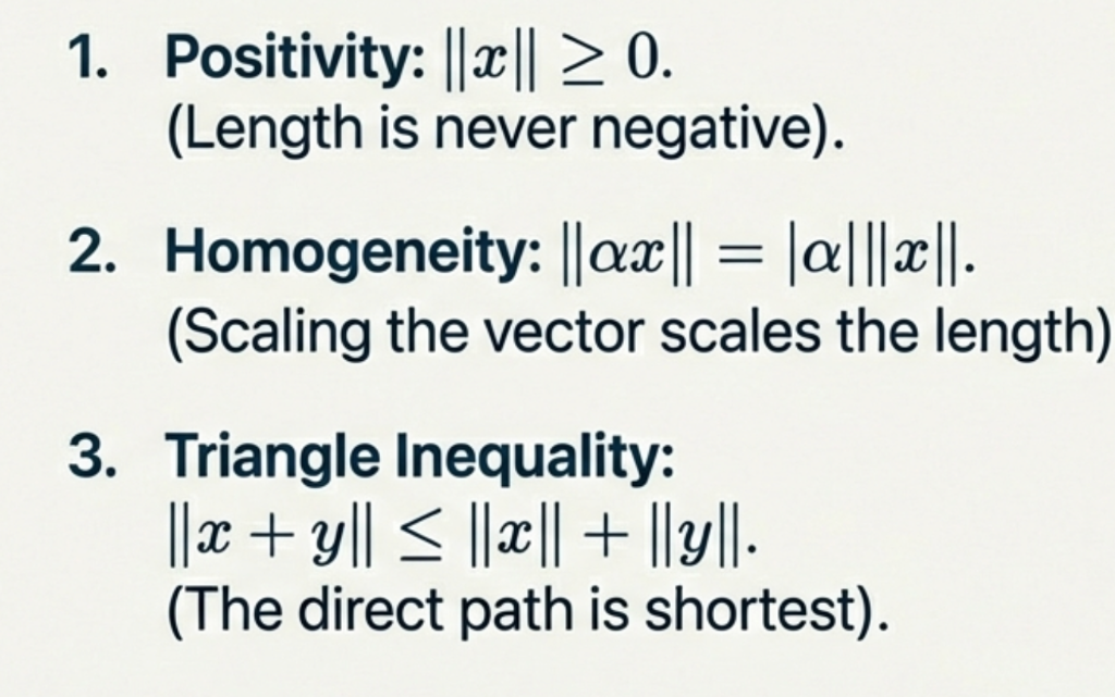
Triangle inequality

Common Norms in \(\mathbb{R}^n\)

Euclidean (\(\ell_2\)) – Most common in ML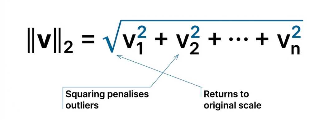

Manhattan (\(\ell_1\)) – Used in regularization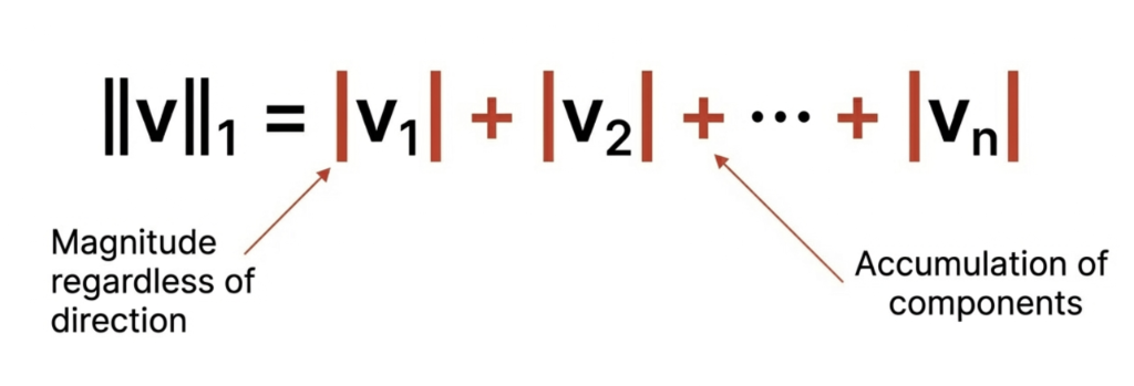

Supremum (\(\ell_\infty\)) – Largest component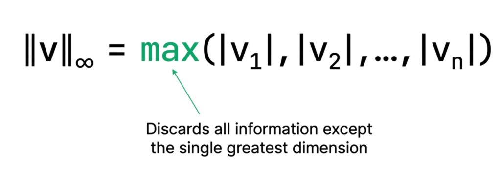

L1 vs L2 distance comparison

Visualizing the Unit Ball

Visualising the ‘Unit Ball’ (points where distance is 1) for different norms.

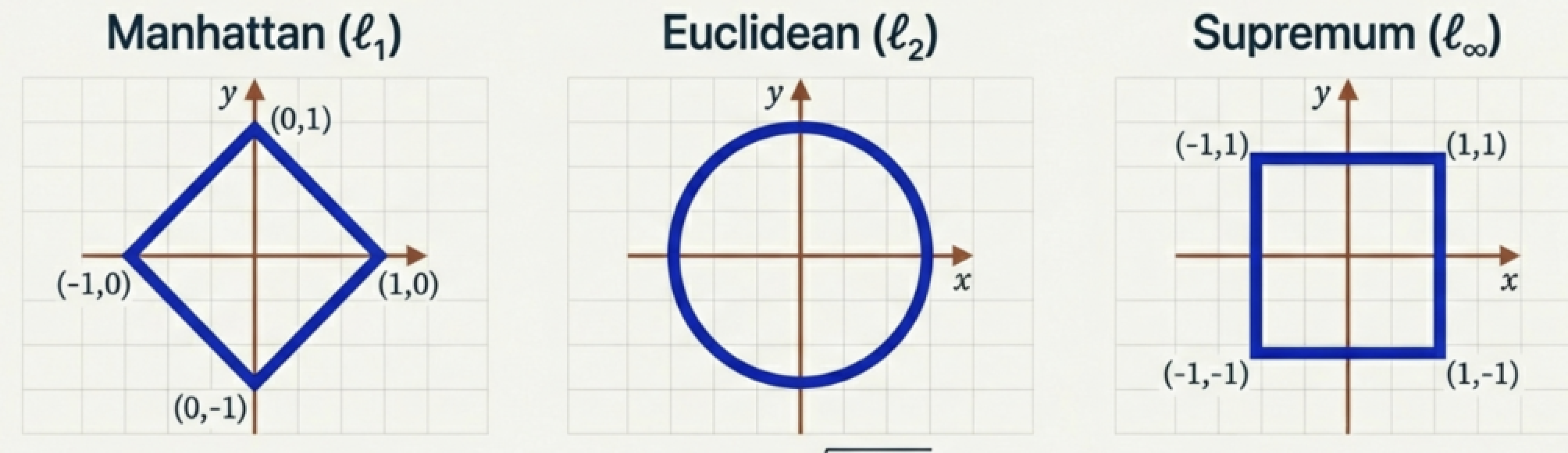
• Manhattan (\(\ell_1\)): Diamond shape
• Euclidean (\(\ell_2\)): Circle (familiar distance)
• Supremum (\(\ell_\infty\)): Square

Unit Vectors (Normalization)

A unit vector has length 1:

\[\|\hat{x}\| = 1\]

Normalization converts any vector to a unit vector:

\[\hat{x} = \frac{x}{\|x\|}\]

Why normalize?

• Focus on direction, not magnitude
  
• Numerical stability
  
• Cosine similarity (angles only)
  
• Neural network inputs

Example:

\[x = \begin{bmatrix} 3 \\ 4 \end{bmatrix}, \quad \|x\| = 5\]

\[\hat{x} = \frac{1}{5}\begin{bmatrix} 3 \\ 4 \end{bmatrix} = \begin{bmatrix} 0.6 \\ 0.8 \end{bmatrix}\]

Check: \(\|\hat{x}\| = \sqrt{0.6^2 + 0.8^2} = 1\) ✓

Distance from Norms

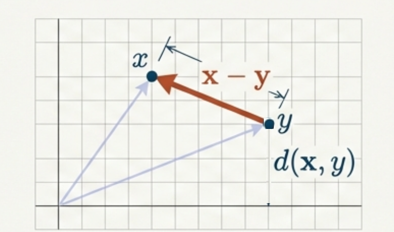
Given a norm, define distance:

\[d(x,y) = \|x - y\|\]

Properties:

• Nonnegative
• Symmetric
• Triangle inequality:
  \(d(x,z) \leq d(x,y) + d(y,z)\)

Distance = length of displacement

Exercise: Calculating Norms

Let \(\mathbf{x} = \begin{bmatrix} 3 \\ -4 \end{bmatrix}\). Calculate:

1. L1 Norm (\(\ell_1\)): \(\|\mathbf{x}\|_1\)
   Answer: 7

   (\(|3| + |-4| = 3 + 4\))
2. L2 Norm (\(\ell_2\)): \(\|\mathbf{x}\|_2\)
   Answer: 5

   (\(\sqrt{3^2 + (-4)^2} = \sqrt{25}\))
3. L-infinity Norm (\(\ell_\infty\)): \(\|\mathbf{x}\|_\infty\)
   Answer: 4

   (\(\max(|3|, |-4|) = 4\))

TABLE OF CONTENTS

1. Introduction✓

2. Tool 1: Norms and Distance✓

3. Tools 2: Inner Products●

4. Tools 3: Orthogonality and Projections○

5. Orthonormal Bases○

6. Matrix Properties○

• What is the Determinant?

• What is a Matrix Inverse?

• Change of Basis

10. Gram–Schmidt Algorithm○

Inner Products: Measuring Similarity

An inner product is a function \(\langle \cdot, \cdot \rangle : V \times V \to \mathbb{R}\) satisfying:

Definition properties:

• Linearity
  e.g., \(\langle \alpha x , y \rangle = \alpha\langle x,y \rangle = \langle x,\alpha y \rangle\)

• Symmetry
  e.g., \(\langle x,y \rangle = \langle y,x \rangle\)

• Positive Definiteness
  e.g., \(\langle x,x \rangle \ge 0\) ; \(\langle x,x \rangle = 0 \iff x = 0\)

The Standard Dot Product:

\[\langle x, y \rangle = \sum_i x_i y_i = \|x\|\|y\|\cos(\theta)\]

Inner product between vector and itself is the norm squared!

Connecting Inner Products to Norms

Inner products naturally give us a way to measure length. We call this the Induced Norm.

\[ \|x\| = \sqrt{\langle x, x \rangle} \]

Example: Using the standard dot product \(\langle x, y \rangle = \sum x_i y_i\):

\[ \|x\| = \sqrt{x \cdot x} = \sqrt{\sum x_i^2} \]

This recovers the Euclidean Norm!

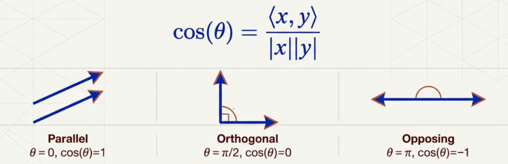
Angles and Similarity

Defined via:

\[\cos(\theta) = \frac{\langle x,y \rangle}{\|x\|\,\|y\|}\]

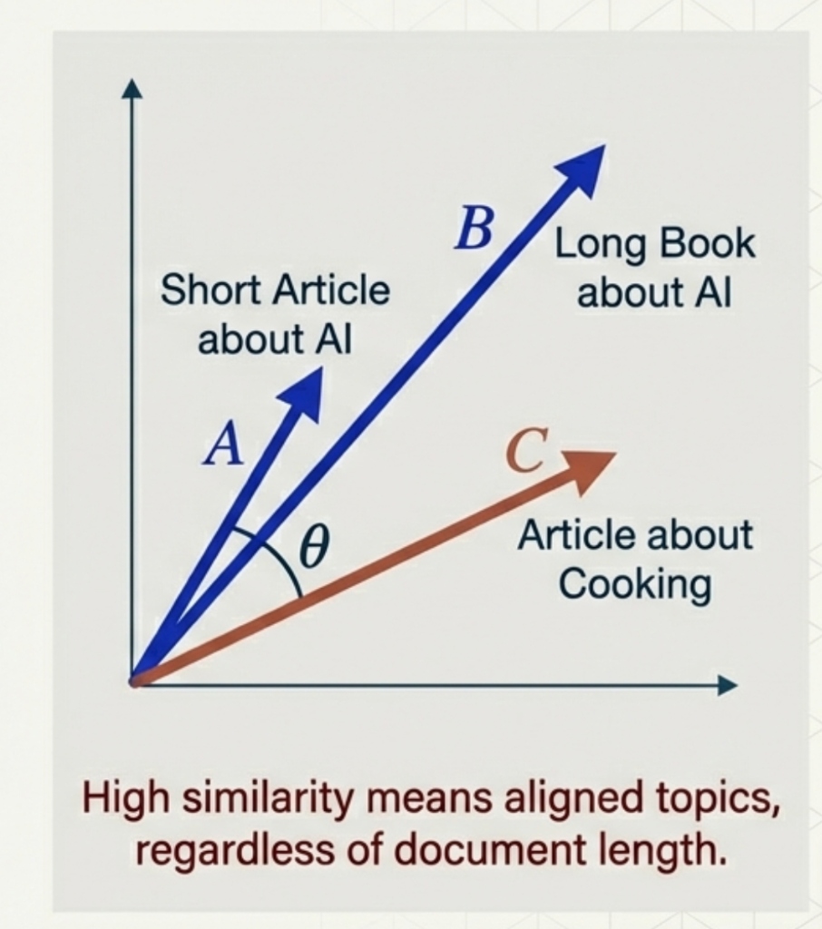
Cosine Similarity

In high-dimensional spaces (like text analysis), we often care about direction, not magnitude.

\[\text{Cosine Similarity} = \frac{\langle x, y \rangle}{\|x\| \|y\|}\]

Exercise: Inner Products & Angles

Consider \(\mathbf{u} = \begin{bmatrix} 1 \\ 5 \end{bmatrix}\) and \(\mathbf{v} = \begin{bmatrix} 5 \\ -1 \end{bmatrix}\).

1. Compute the dot product \(\langle \mathbf{u}, \mathbf{v} \rangle\).
   Answer: 0

   (\(1(5) + 5(-1) = 5 - 5\))
2. What is the angle between them?
   Answer: 90° (Orthogonal)

   (Since dot product is 0)

TABLE OF CONTENTS

1. Introduction✓

2. Tool 1: Norms and Distance✓

3. Tools 2: Inner Products✓

4. Tools 3: Orthogonality and Projections●

5. Orthonormal Bases○

6. Matrix Properties○

• What is the Determinant?

• What is a Matrix Inverse?

• Change of Basis

10. Gram–Schmidt Algorithm○

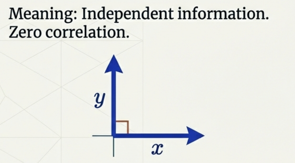
Orthogonality

Two vectors are orthogonal if:

\[\langle x,y \rangle = 0\]

Interpretation:

• No shared information
• Independent directions
• Perpendicular in geometric space

Projection of One Vector onto Another

Scalar projection (length of projection):

\[\text{comp}_y(x) = \|x\|\cos(\theta) = \frac{\langle x,y \rangle}{\|y\|}\]

Vector projection (actual vector):

\[\mathrm{proj}_y(x) = \frac{\langle x,y \rangle}{\|y\|^2} y = \frac{\langle x,y \rangle}{\langle y,y \rangle} y\]

Used in:

• Feature extraction
• PCA

Vector and Scalar Projections

Exercise: Projections in \(\mathbb{R}^3\)

Project vector \(\mathbf{b} = \begin{bmatrix} 2 \\ 4 \\ 1 \end{bmatrix}\) onto \(\mathbf{a} = \begin{bmatrix} 1 \\ 1 \\ 0 \end{bmatrix}\).

1. Scalar Projection (\(\frac{\mathbf{b} \cdot \mathbf{a}}{\|\mathbf{a}\|}\)):

Answer: \(3\sqrt{2} \approx 4.24\) (\(\mathbf{b}\cdot\mathbf{a}=6\), \(\|\mathbf{a}\|=\sqrt{2}\))

2. Vector Projection (\(\text{proj}_\mathbf{a} \mathbf{b}\)):

Answer:

\(\begin{bmatrix} 3 \\ 3 \\ 0 \end{bmatrix}\)

TABLE OF CONTENTS

1. Introduction✓

2. Tool 1: Norms and Distance✓

3. Tools 2: Inner Products✓

4. Tools 3: Orthogonality and Projections✓

5. Orthonormal Bases●

6. Matrix Properties○

• What is the Determinant?

• What is a Matrix Inverse?

• Change of Basis

10. Gram–Schmidt Algorithm○

Orthonormal Bases

A basis \(\{v_i\}\) is orthonormal if every vector has unit length and all are mutually orthogonal.

Conditions:

1. \(\|v_i\| = 1\)
2. \(\langle v_i, v_j \rangle = 0\) for \(i \neq j\)

Why use orthonormal bases?

• Coordinates are easy: Direct projection (\(x_i = \langle x, v_i \rangle\))
• Norms are simple: Pythagorean theorem holds (\(\|x\|^2 = \sum x_i^2\))
• Computations decouple: Each dimension is independent

Standard orthonormal basis in \(\mathbb{R}^3\)

Exercise: Orthonormal Basis

Is the set \(S\) an orthonormal basis for \(\mathbb{R}^2\)?

\(S = \left\{ \begin{bmatrix} \frac{1}{\sqrt{2}} \\ \frac{1}{\sqrt{2}} \end{bmatrix}, \begin{bmatrix} \frac{1}{\sqrt{2}} \\ -\frac{1}{\sqrt{2}} \end{bmatrix} \right\}\)

Check Conditions:

1. Unit Length? Yes.
   \((\frac{1}{\sqrt{2}})^2 + (\frac{1}{\sqrt{2}})^2 = \frac{1}{2} + \frac{1}{2} = 1\)
2. Orthogonal? Yes.
   \(\frac{1}{\sqrt{2}}(\frac{1}{\sqrt{2}}) + \frac{1}{\sqrt{2}}(-\frac{1}{\sqrt{2}}) = \frac{1}{2} - \frac{1}{2} = 0\)

Conclusion: Yes, it is an orthonormal basis!

TABLE OF CONTENTS

1. Introduction✓

2. Tool 1: Norms and Distance✓

3. Tools 2: Inner Products✓

4. Tools 3: Orthogonality and Projections✓

5. Orthonormal Bases✓

6. Matrix Properties●

• What is the Determinant?

• What is a Matrix Inverse?

• Change of Basis

10. Gram–Schmidt Algorithm○

What is the Determinant?

Watch how different transformations change the area of the unit square!

What is the Determinant?

The determinant measures how much a transformation scales area.

For a 2×2 matrix: \[\det\begin{pmatrix} a & b \\ c & d \end{pmatrix} = ad - bc\]

Geometric Meaning:

• Start with a unit square (area = 1)
• Apply matrix transformation
• New area = \(|\det(A)|\)

Quick Examples:

Matrix	det	Area Factor
\(\begin{pmatrix} 2 & 0 \\ 0 & 3 \end{pmatrix}\)	6	6× bigger
\(\begin{pmatrix} 1 & 1 \\ 0 & 1 \end{pmatrix}\)	1	Same area
\(\begin{pmatrix} 2 & 4 \\ 1 & 2 \end{pmatrix}\)	0	Collapsed!

The determinant tells you how the transformation scales space!

What the Sign Tells Us

det > 0

✅ Orientation Preserved

The “handedness” stays the same (counterclockwise stays counterclockwise)

det < 0

🔄 Orientation Flipped

Like looking in a mirror — left becomes right

det = 0

💀 Space Collapsed

2D → 1D line (or point). Matrix is singular — no inverse!

det = 0 means the transformation loses information — you can’t undo it!

Computing Determinants in NumPy

import numpy as np

#> Define matrices
A = np.array([[2, 0], 
              [0, 3]])    # Scaling matrix

B = np.array([[1, 2], 
              [3, 4]])    # General matrix

C = np.array([[2, 4], 
              [1, 2]])    # Singular matrix (det = 0)

#> Compute determinants
print(f"det(A) = {np.linalg.det(A):.2f}")  #> Expected: 6
print(f"det(B) = {np.linalg.det(B):.2f}")  #> Expected: -2
print(f"det(C) = {np.linalg.det(C):.2f}")  #> Expected: 0

det(A) = 6.00
det(B) = -2.00
det(C) = 0.00

Use np.linalg.det(A) to compute the determinant of any matrix!

What is a Matrix Inverse?

Definition: The inverse \(A^{-1}\) “undoes” the transformation \(A\):

\[A A^{-1} = A^{-1} A = I\]

Geometric Intuition:

• Rotation by 30° → Inverse rotates by -30°
• Scaling by 2 → Inverse scales by 0.5
• Shear → Inverse shears the opposite way

2×2 Inverse Formula:

\[A = \begin{pmatrix} a & b \\ c & d \end{pmatrix} \Rightarrow A^{-1} = \frac{1}{\det(A)} \begin{pmatrix} d & -b \\ -c & a \end{pmatrix}\]

Key Insight: Swap \(a \leftrightarrow d\), negate \(b\) and \(c\), divide by determinant.

The inverse only exists when det(A) ≠ 0!

Matrix Inverse: Example

Given: \[A = \begin{pmatrix} 3 & 1 \\ 2 & 4 \end{pmatrix}\]

Step 1: Calculate determinant \[\det(A) = 3 \times 4 - 1 \times 2 = 12 - 2 = 10\]

Step 2: Apply the formula (swap, negate, divide) \[A^{-1} = \frac{1}{10} \begin{pmatrix} 4 & -1 \\ -2 & 3 \end{pmatrix} = \begin{pmatrix} 0.4 & -0.1 \\ -0.2 & 0.3 \end{pmatrix}\]

Step 3: Verify: \(A \cdot A^{-1} = I\)

Always verify your inverse by checking that \(A \cdot A^{-1} = I\)!

Computing Inverses in NumPy

import numpy as np
#> Define a matrix  
A = np.array([[3, 1], 
              [2, 4]])
#> Compute inverse
A_inv = np.linalg.inv(A)
print("\nA^(-1) =\n", A_inv)

#> Verify: A @ A_inv = I
print("\nA @ A^(-1) =\n", A @ A_inv)

A^(-1) =
 [[ 0.4 -0.1]
 [-0.2  0.3]]

A @ A^(-1) =
 [[1. 0.]
 [0. 1.]]

Use np.linalg.inv(A) — but only if you really need the inverse!

Change of Basis

Why Change Basis?

Different coordinate systems describe the same vector differently.

Example: A point at \((3, 2)\) in standard coordinates might be \((1, 1)\) in a rotated coordinate system!

Same point in space, different numbers to describe it!

The Change of Basis Formula

If \(B\) contains new basis vectors as columns:

To convert TO new basis: \[[\mathbf{v}]_{\text{new}} = B^{-1} [\mathbf{v}]_{\text{standard}}\]

To convert FROM new basis: \[[\mathbf{v}]_{\text{standard}} = B [\mathbf{v}]_{\text{new}}\]

Key Insight: \(B^{-1}\) converts TO the new basis, \(B\) converts FROM it.

The inverse of a basis matrix converts coordinates between systems!

Change of Basis: Example

Problem: Convert \(\mathbf{v} = \begin{pmatrix} 4 \\ 3 \end{pmatrix}\) to a stretched basis.

New basis: \(\mathbf{b}_1 = \begin{pmatrix} 2 \\ 0 \end{pmatrix}\), \(\mathbf{b}_2 = \begin{pmatrix} 0 \\ 1 \end{pmatrix}\)

Step 1: Build basis matrix \(B = \begin{pmatrix} 2 & 0 \\ 0 & 1 \end{pmatrix}\)

Step 2: Find inverse \(B^{-1} = \begin{pmatrix} 0.5 & 0 \\ 0 & 1 \end{pmatrix}\)

Step 3: Convert: \([\mathbf{v}]_{\text{new}} = B^{-1} \mathbf{v} = \begin{pmatrix} 2 \\ 3 \end{pmatrix}\)

The point (4,3) in standard coords = (2,3) in the stretched basis!

Exercise: Change of Basis

🧮 Practice Problem

Given: New basis vectors \(\mathbf{b}_1 = \begin{pmatrix} 1 \\ 1 \end{pmatrix}\) and \(\mathbf{b}_2 = \begin{pmatrix} -1 \\ 1 \end{pmatrix}\)

Convert: \(\mathbf{v} = \begin{pmatrix} 2 \\ 4 \end{pmatrix}\) to the new basis.

Solution:

\(B = \begin{pmatrix} 1 & -1 \\ 1 & 1 \end{pmatrix}\), \(\det(B) = 2\)

\(B^{-1} = \frac{1}{2}\begin{pmatrix} 1 & 1 \\ -1 & 1 \end{pmatrix}\)

\([\mathbf{v}]_{\text{new}} = B^{-1}\mathbf{v} = \begin{pmatrix} 3 \\ 1 \end{pmatrix}\)

TABLE OF CONTENTS

1. Introduction✓

2. Tool 1: Norms and Distance✓

3. Tools 2: Inner Products✓

4. Tools 3: Orthogonality and Projections✓

5. Orthonormal Bases✓

6. Matrix Properties✓

• What is the Determinant?

• What is a Matrix Inverse?

• Change of Basis

10. Gram–Schmidt Algorithm●

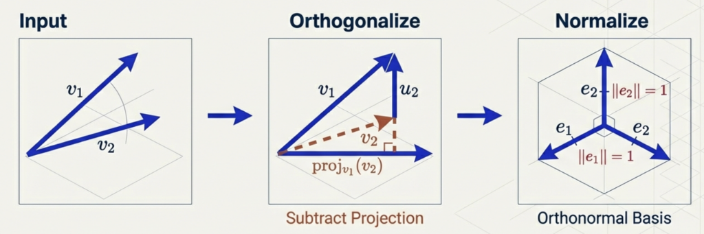
Gram–Schmidt Orthogonalization

Goal:
Convert any linearly independent set into an orthonormal basis

Algorithm:

1. Start with basis
2. Orthogonalize
3. Normalize

Applications: Why Gram–Schmidt?

Setup: Predicting House Price using two features:

1. \(x_1\): House Size (\(m^2\))
2. \(x_2\): Number of Rooms

The Problem: These are highly correlated! (Bigger house \(\to\) more rooms).

• Model Confusion: Which feature actually explains the price?

The Solution (Gram–Schmidt): Create a new feature \(x_2^\perp\): \[x_2^\perp = x_2 - \text{proj}_{x_1}(x_2)\] “Rooms that CANNOT be explained by Size”

Now \(x_1\) and \(x_2^\perp\) are orthogonal. The model becomes stable and interpretable.

Gram–Schmidt (Step Form)

Given input basis \(u_1,\dots,u_n\):

1. \(v_1 = u_1\)
2. \(v_2 = u_2 - \mathrm{proj}_{v_1}(u_2)\)
3. \(v_3 = u_3 - \mathrm{proj}_{v_1}(u_3) - \mathrm{proj}_{v_2}(u_3)\)
4. Continue…
5. Normalize all \(v_i\) to get \(e_i = v_i / \|v_i\|\)

Exercise: Gram–Schmidt Process

Convert \(u_1 = \begin{bmatrix} 1 \\ 1 \end{bmatrix}, u_2 = \begin{bmatrix} 1 \\ 0 \end{bmatrix}\) into an orthonormal basis.

1. Step 1 (\(v_1\)):

   \[v_1 = u_1 = \begin{bmatrix} 1 \\ 1 \end{bmatrix}\]

2. Step 2 (\(v_2\)):

   \[v_2 = u_2 - \frac{u_2 \cdot v_1}{v_1 \cdot v_1} v_1 = \begin{bmatrix} 1 \\ 0 \end{bmatrix} - \frac{1}{2} \begin{bmatrix} 1 \\ 1 \end{bmatrix} = \begin{bmatrix} 0.5 \\ -0.5 \end{bmatrix}\]

3. Step 3 (Normalize):

   \[e_1 = \begin{bmatrix} \frac{1}{\sqrt{2}} \\ \frac{1}{\sqrt{2}} \end{bmatrix}, \quad e_2 = \begin{bmatrix} \frac{1}{\sqrt{2}} \\ -\frac{1}{\sqrt{2}} \end{bmatrix}\]

Gram–Schmidt in Python (Using Libraries)

In practice, we use QR Decomposition (numerically stable):

import numpy as np

#> X is our data matrix (features as columns)
#> Q will be the orthonormal basis
#> R will be the upper triangular matrix
Q, R = np.linalg.qr(X)

Visualizing Decorrelation (Sparsity of Correlations):

Before (\(X^T X\))

High Values Everywhere
(Correlated)
⬛️ ⬛️ ⬛️
⬛️ ⬛️ ⬛️
⬛️ ⬛️ ⬛️

\(\to\)

After (\(Q^T Q\))

Diagonal / Sparse
(Identity Matrix)
🟩 ⬜️ ⬜️
⬜️ 🟩 ⬜️
⬜️ ⬜️ 🟩

Important Caveat

• If inputs are linearly dependent
• Gram–Schmidt produces a zero vector

This reveals dependence automatically!

Thank You!